
Expected goals has become one of the most important concepts in modern football analytics. Instead of judging a team only by goals scored, xG helps us estimate the quality of the chances created. In this tutorial, we will build a practical expected goals model in R using football data, feature engineering, logistic regression, model evaluation, and visualization.
This is a hands-on guide for analysts who want to move beyond simple football statistics and start building reproducible soccer analytics workflows in R.
What Is Expected Goals?
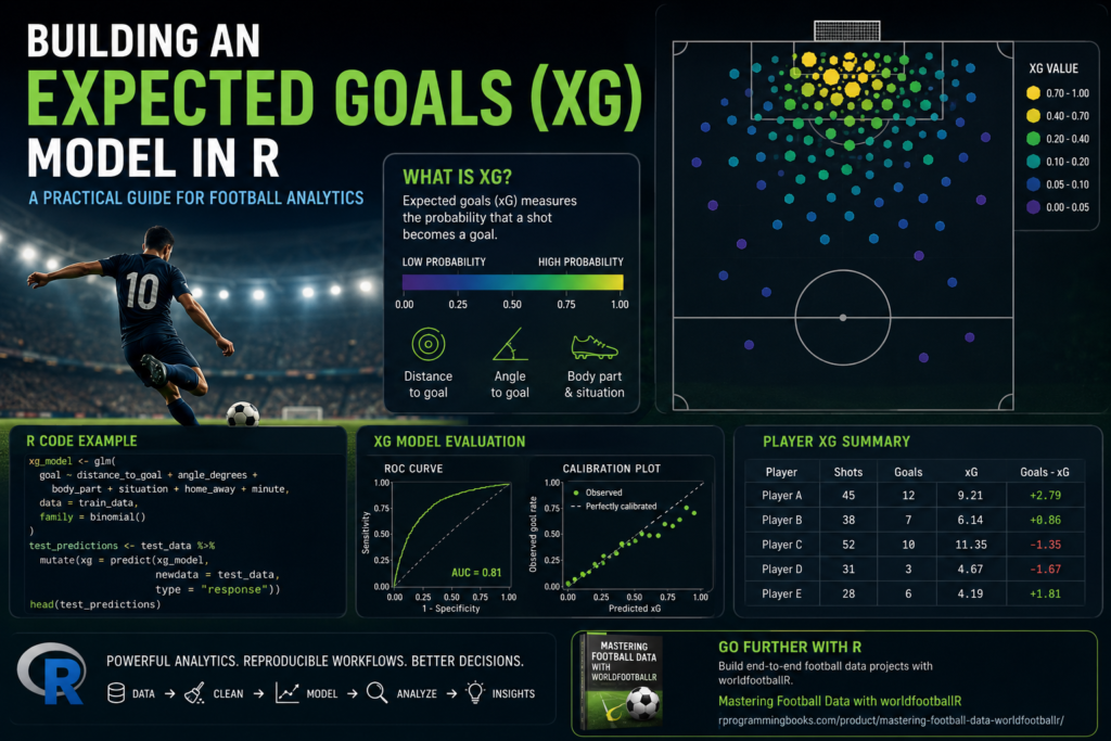
Expected goals, usually written as xG, measures the probability that a shot becomes a goal. A shot from two meters in front of goal will usually have a high xG value, while a long-range shot from outside the box will usually have a low xG value.
An xG model can use variables such as:
- Shot distance
- Shot angle
- Body part used
- Game state
- Minute of the match
- Shot type
- Set-piece situation
- Home or away context
In this post, we will build a clean starter model using R. You can later extend it with richer event data, tracking data, or more advanced machine learning models.
Install and Load R Packages
# Core data science packages
install.packages(c(
  "tidyverse",
  "ggplot2",
  "dplyr",
  "readr",
  "janitor",
  "broom",
  "yardstick",
  "rsample",
  "pROC",
  "patchwork"
))

# Football data package
install.packages("worldfootballR")

library(tidyverse)
library(ggplot2)
library(dplyr)
library(readr)
library(janitor)
library(broom)
library(yardstick)
library(rsample)
library(pROC)
library(patchwork)
library(worldfootballR)
Create a Simple Shot Dataset
Different public football data sources structure shot data differently. To make this tutorial reproducible, we will first create a synthetic shot dataset that behaves like real football event data. Later, you can replace this with your own data from FBref, StatsBomb open data, Wyscout-style exports, or custom event feeds.
set.seed(123)

n_shots <- 5000

shots <- tibble(
  shot_id = 1:n_shots,
  player = sample(
    c("Player A", "Player B", "Player C", "Player D", "Player E"),
    n_shots,
    replace = TRUE
  ),
  team = sample(
    c("Team Red", "Team Blue", "Team Green", "Team White"),
    n_shots,
    replace = TRUE
  ),
  minute = sample(1:95, n_shots, replace = TRUE),
  x_location = runif(n_shots, min = 70, max = 120),
  y_location = runif(n_shots, min = 0, max = 80),
  body_part = sample(
    c("Right Foot", "Left Foot", "Header", "Other"),
    n_shots,
    replace = TRUE,
    prob = c(0.43, 0.32, 0.20, 0.05)
  ),
  situation = sample(
    c("Open Play", "Corner", "Free Kick", "Penalty", "Counter Attack"),
    n_shots,
    replace = TRUE,
    prob = c(0.68, 0.12, 0.08, 0.03, 0.09)
  ),
  home_away = sample(c("Home", "Away"), n_shots, replace = TRUE)
)

glimpse(shots)
Engineer Shot Distance and Angle
Distance and angle are two of the most important features in a basic xG model. We will assume the goal is centered at x = 120 and y = 40.
goal_x <- 120
goal_y <- 40

shots <- shots %>%
  mutate(
    distance_to_goal = sqrt(
      (goal_x - x_location)^2 + (goal_y - y_location)^2
    ),
    angle_to_goal = atan2(
      abs(goal_y - y_location),
      goal_x - x_location
    ),
    angle_degrees = angle_to_goal * 180 / pi
  )

shots %>%
  select(shot_id, x_location, y_location, distance_to_goal, angle_degrees) %>%
  head()
Create a Goal Outcome
For demonstration, we will simulate goals using realistic football logic. Shots closer to goal should be more likely to become goals. Penalties should have higher probability. Headers and long-range attempts should usually be harder.
shots <- shots %>%
  mutate(
    linear_probability =
      -2.8 -
      0.08 * distance_to_goal +
      0.025 * angle_degrees +
      if_else(body_part == "Header", -0.35, 0) +
      if_else(body_part == "Other", -0.60, 0) +
      if_else(situation == "Penalty", 3.00, 0) +
      if_else(situation == "Counter Attack", 0.35, 0) +
      if_else(situation == "Free Kick", -0.45, 0),

    goal_probability = plogis(linear_probability),
    goal = rbinom(n(), size = 1, prob = goal_probability)
  )

shots %>%
  summarise(
    total_shots = n(),
    total_goals = sum(goal),
    conversion_rate = mean(goal)
  )
Explore the Shot Data
shots %>%
  count(body_part, goal) %>%
  group_by(body_part) %>%
  mutate(rate = n / sum(n))
shots %>%
group_by(situation) %>%
summarise(
shots = n(),
goals = sum(goal),
conversion_rate = mean(goal),
avg_distance = mean(distance_to_goal),
.groups = "drop"
) %>%
arrange(desc(conversion_rate))Visualize Shot Locations
ggplot(shots, aes(x = x_location, y = y_location, color = factor(goal))) +
  geom_point(alpha = 0.35) +
  coord_fixed() +
  labs(
    title = "Shot Map",
    x = "Pitch Length",
    y = "Pitch Width",
    color = "Goal"
  ) +
  theme_minimal()
Split Data into Training and Testing Sets
set.seed(123)

shot_split <- initial_split(shots, prop = 0.80, strata = goal)

train_data <- training(shot_split)
test_data  <- testing(shot_split)

nrow(train_data)
nrow(test_data)
Build a Logistic Regression xG Model
Expected goals is naturally suited to logistic regression because the outcome is binary: goal or no goal.
xg_model <- glm(
  goal ~ distance_to_goal +
    angle_degrees +
    body_part +
    situation +
    home_away +
    minute,
  data = train_data,
  family = binomial()
)

summary(xg_model)
Convert Model Output into xG Values
test_predictions <- test_data %>%
  mutate(
    xg = predict(xg_model, newdata = test_data, type = "response")
  )

test_predictions %>%
  select(player, team, goal, xg, distance_to_goal, angle_degrees) %>%
  head(10)
Evaluate the xG Model
A good xG model should not only predict goals, but also produce well-calibrated probabilities. If 100 shots each have an xG of 0.10, we would expect roughly 10 goals over a large enough sample.
test_predictions %>%
  summarise(
    actual_goals = sum(goal),
    expected_goals = sum(xg),
    avg_xg = mean(xg),
    actual_conversion = mean(goal)
  )
ROC AUC
roc_obj <- roc(
  response = test_predictions$goal,
  predictor = test_predictions$xg
)

auc(roc_obj)
plot(
roc_obj,
main = "ROC Curve for xG Model"
)Brier Score
brier_score <- mean((test_predictions$xg - test_predictions$goal)^2)

brier_score
Create xG Buckets for Calibration
calibration_table <- test_predictions %>%
  mutate(
    xg_bucket = cut(
      xg,
      breaks = seq(0, 1, by = 0.05),
      include.lowest = TRUE
    )
  ) %>%
  group_by(xg_bucket) %>%
  summarise(
    shots = n(),
    avg_xg = mean(xg),
    actual_goal_rate = mean(goal),
    goals = sum(goal),
    .groups = "drop"
  ) %>%
  filter(shots >= 10)

calibration_table
ggplot(calibration_table, aes(x = avg_xg, y = actual_goal_rate)) +
geom_point(size = 3) +
geom_abline(intercept = 0, slope = 1, linetype = "dashed") +
labs(
title = "xG Model Calibration",
x = "Average Predicted xG",
y = "Actual Goal Rate"
) +
theme_minimal()Player-Level xG Analysis
Once every shot has an xG value, we can aggregate by player. This allows us to compare goals, expected goals, overperformance, and shot volume.
player_xg <- test_predictions %>%
  group_by(player) %>%
  summarise(
    shots = n(),
    goals = sum(goal),
    xg = sum(xg),
    goals_minus_xg = goals - xg,
    xg_per_shot = mean(xg),
    conversion_rate = mean(goal),
    .groups = "drop"
  ) %>%
  arrange(desc(xg))

player_xg
ggplot(player_xg, aes(x = reorder(player, xg), y = xg)) +
geom_col() +
coord_flip() +
labs(
title = "Expected Goals by Player",
x = "Player",
y = "Total xG"
) +
theme_minimal()Team-Level xG Analysis
team_xg <- test_predictions %>%
  group_by(team) %>%
  summarise(
    shots = n(),
    goals = sum(goal),
    xg = sum(xg),
    goals_minus_xg = goals - xg,
    avg_xg_per_shot = mean(xg),
    .groups = "drop"
  ) %>%
  arrange(desc(xg))

team_xg
ggplot(team_xg, aes(x = reorder(team, goals_minus_xg), y = goals_minus_xg)) +
geom_col() +
coord_flip() +
labs(
title = "Goals Minus xG by Team",
x = "Team",
y = "Goals - Expected Goals"
) +
theme_minimal()Shot Quality Distribution
ggplot(test_predictions, aes(x = xg)) +
  geom_histogram(bins = 40) +
  labs(
    title = "Distribution of Shot Quality",
    x = "Expected Goals",
    y = "Number of Shots"
  ) +
  theme_minimal()
Compare Goals and xG by Situation
situation_xg <- test_predictions %>%
  group_by(situation) %>%
  summarise(
    shots = n(),
    goals = sum(goal),
    xg = sum(xg),
    avg_xg = mean(xg),
    .groups = "drop"
  ) %>%
  arrange(desc(avg_xg))

situation_xg
situation_long <- situation_xg %>%
select(situation, goals, xg) %>%
pivot_longer(
cols = c(goals, xg),
names_to = "metric",
values_to = "value"
)
ggplot(situation_long, aes(x = reorder(situation, value), y = value, fill = metric)) +
geom_col(position = "dodge") +
coord_flip() +
labs(
title = "Goals vs Expected Goals by Situation",
x = "Situation",
y = "Value",
fill = "Metric"
) +
theme_minimal()Build a More Advanced xG Model with Interactions
A simple model is useful, but football is full of interactions. For example, distance may affect headers differently than footed shots. We can include interaction terms in the model.
xg_model_interaction <- glm(
  goal ~ distance_to_goal * body_part +
    angle_degrees +
    situation +
    home_away +
    minute,
  data = train_data,
  family = binomial()
)

summary(xg_model_interaction)
test_predictions_interaction <- test_data %>%
mutate(
xg_interaction = predict(
xg_model_interaction,
newdata = test_data,
type = "response"
)
)
mean((test_predictions_interaction$xg_interaction - test_predictions_interaction$goal)^2)Compare Two xG Models
model_comparison <- tibble(
  model = c("Basic Logistic Regression", "Interaction Logistic Regression"),
  brier_score = c(
    mean((test_predictions$xg - test_predictions$goal)^2),
    mean((test_predictions_interaction$xg_interaction - test_predictions_interaction$goal)^2)
  ),
  total_predicted_goals = c(
    sum(test_predictions$xg),
    sum(test_predictions_interaction$xg_interaction)
  ),
  actual_goals = c(
    sum(test_predictions$goal),
    sum(test_predictions_interaction$goal)
  )
)

model_comparison
Create a Reusable xG Prediction Function
predict_xg <- function(model, new_shots) {
  new_shots %>%
    mutate(
      predicted_xg = predict(
        model,
        newdata = new_shots,
        type = "response"
      )
    )
}

new_predictions <- predict_xg(xg_model, test_data)

head(new_predictions)
Create a Custom Shot Example
custom_shot <- tibble(
  distance_to_goal = 12,
  angle_degrees = 28,
  body_part = "Right Foot",
  situation = "Open Play",
  home_away = "Home",
  minute = 62
)

predict(
  xg_model,
  newdata = custom_shot,
  type = "response"
)
Use worldfootballR for Real Football Workflows
For real projects, you can use packages such as worldfootballR to collect football data from public sources and build reproducible analysis pipelines. The exact available columns depend on the source and endpoint, so always inspect your data before modeling.
library(worldfootballR)
library(tidyverse)

# Example: get FBref match results
# Adjust country, gender, season_end_year, and tier depending on your project

premier_league_results <- fb_match_results(
  country = "ENG",
  gender = "M",
  season_end_year = 2025,
  tier = "1st"
)

glimpse(premier_league_results)
premier_league_results %>%
clean_names() %>%
head()If you are building a full football analytics pipeline with FBref, Transfermarkt, and Understat-style workflows, a more structured project template can save a lot of time. I cover that type of end-to-end workflow in Mastering Football Data with worldfootballR, especially for readers who want reusable R scripts, clean folders, and practical football data examples.
Example: Clean Match Results Data
clean_results <- premier_league_results %>%
  clean_names()

clean_results %>%
  glimpse()
# Example structure will depend on the returned data
# Always check column names first
names(clean_results)Build a Match-Level Team Summary
# This is an example pattern.
# You may need to adjust column names depending on your data source.

team_summary_example <- clean_results %>%
  summarise(
    matches = n()
  )

team_summary_example
Save Your xG Model
Once you have trained a model, save it so you can reuse it later in reports, dashboards, APIs, or automated pipelines.
saveRDS(xg_model, "xg_model_logistic_regression.rds")

loaded_xg_model <- readRDS("xg_model_logistic_regression.rds")

predict(
  loaded_xg_model,
  newdata = custom_shot,
  type = "response"
)
Create an xG Report Table
xg_report <- test_predictions %>%
  group_by(team, player) %>%
  summarise(
    shots = n(),
    goals = sum(goal),
    xg = round(sum(xg), 2),
    goals_minus_xg = round(goals - sum(xg), 2),
    xg_per_shot = round(mean(xg), 3),
    .groups = "drop"
  ) %>%
  arrange(desc(xg))

xg_report
write_csv(xg_report, "xg_player_report.csv")Create an xG Shot Map
ggplot(test_predictions, aes(x = x_location, y = y_location)) +
  geom_point(aes(size = xg, alpha = xg)) +
  coord_fixed() +
  labs(
    title = "xG Shot Map",
    x = "Pitch Length",
    y = "Pitch Width",
    size = "xG",
    alpha = "xG"
  ) +
  theme_minimal()
Create a High-Value Chances Table
big_chances <- test_predictions %>%
  filter(xg >= 0.30) %>%
  arrange(desc(xg)) %>%
  select(
    player,
    team,
    minute,
    body_part,
    situation,
    distance_to_goal,
    angle_degrees,
    xg,
    goal
  )

big_chances %>%
  head(20)
Model Improvement Ideas
This starter xG model can be improved in many ways. A professional football analytics workflow may include:
- More accurate shot coordinates
- Goalkeeper position
- Defender pressure
- Pass type before the shot
- Through balls and cutbacks
- Shot speed
- First-time shots
- Game state
- Team strength
- Player finishing history
Train an XGBoost-Style Model Later
Logistic regression is interpretable and a good starting point. For higher predictive performance, you can later compare it with random forests, gradient boosting, or Bayesian models.
# Example packages for future model upgrades
# install.packages(c("xgboost", "ranger", "tidymodels"))

library(tidymodels)

# A future tidymodels workflow could look like this:

xg_recipe <- recipe(
  goal ~ distance_to_goal + angle_degrees + body_part + situation + home_away + minute,
  data = train_data
) %>%
  step_dummy(all_nominal_predictors()) %>%
  step_normalize(all_numeric_predictors())

xg_recipe
Build a Tidymodels Logistic Regression Workflow
logistic_spec <- logistic_reg() %>%
  set_engine("glm") %>%
  set_mode("classification")

xg_workflow <- workflow() %>%
  add_recipe(xg_recipe) %>%
  add_model(logistic_spec)

xg_fit <- fit(
  xg_workflow,
  data = train_data %>%
    mutate(goal = factor(goal, levels = c(0, 1)))
)

xg_fittidy(xg_fit)Predict Probabilities with Tidymodels
tidy_predictions <- predict(
  xg_fit,
  new_data = test_data,
  type = "prob"
) %>%
  bind_cols(test_data %>% mutate(goal = factor(goal, levels = c(0, 1))))

head(tidy_predictions)
tidy_predictions %>%
roc_auc(
truth = goal,
.pred_1
)Turn xG into Match Insights
The real value of expected goals is not just predicting whether one shot becomes a goal. The value comes from aggregation. Once every shot has a probability, you can create match-level and season-level insights.
match_shots <- test_predictions %>%
  mutate(
    match_id = sample(1:100, n(), replace = TRUE)
  )

match_xg <- match_shots %>%
  group_by(match_id, team) %>%
  summarise(
    shots = n(),
    goals = sum(goal),
    xg = sum(xg),
    .groups = "drop"
  )

match_xg %>%
  arrange(match_id, desc(xg)) %>%
  head(20)
Find Teams Creating Better Chances
team_chance_quality <- test_predictions %>%
  group_by(team) %>%
  summarise(
    shots = n(),
    total_xg = sum(xg),
    avg_xg_per_shot = mean(xg),
    big_chances = sum(xg >= 0.30),
    low_quality_shots = sum(xg <= 0.05),
    .groups = "drop"
  ) %>%
  arrange(desc(avg_xg_per_shot))

team_chance_quality
Final Thoughts
Building an expected goals model in R is one of the best ways to learn football analytics because it combines data cleaning, feature engineering, statistical modeling, visualization, and interpretation. A simple logistic regression model can already teach you a lot about shot quality, player performance, and team attacking style.
From here, the next steps are clear: use richer football data, improve your features, compare different models, evaluate calibration, and build repeatable workflows that can be updated every week during the season.
Expected goals is not the final answer to football analysis, but it is one of the best starting points for serious soccer data science in R.